This is the basic GMDH algorithm. It use an input data sample as a matrix containing N levels (points) of observations over a set of M variables. A data sample is divided into two parts. If regularity criterion AR(s) is used, then approximately two-thirds of observations make up the training subsample N_A, and the remaining part of observations (e.g. every third point with same variance) form the test subsample N_B . The training subsample is used to derive estimates for the coefficients of the polynomial, and the test subsample is used to choose the structure of the optimal model, that is one for which the regularity criterion AR(s) takes on a minimal value:

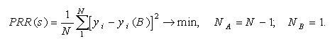
or better to use the cross-validation criterion PRR(s) (it take into account all information in data sample and it can be computed without recalculating of system for each test point). Each point successively is taken as test subsample and then averaged value of criteria is used:

To test a model for compliance with the differential balance criterion, the input data sample is divided into two equal parts. This criterion requires to choose a model that would, as far as possible, be the same on both subsamples. The balance criterion will yield the only optimal physical model solely if the input data are noisy.

To obtain a smooth curve of criterion value, which would permit one to formulate the exhaustive-search termination rule, the full exhaustive search is performed on models classed into groups of an equal complexity. The first layer uses the information contained in every column of the sample; that is the search is applied to partial descriptions of the form

Non-linear members can be taken as new input variables in data sampling. The output variable is specified in this algorithm in advance by the experimenter. For each model system of Gauss normal equations is solved. At the second layer all models-candidates of the following form are sorted:

The models are evaluated for compliance with the criterion, and the procedure is carried on as long as the criterion minimum will be find. To decrease calculation time we recommend now to select at some (6-8) layer a set of the best F variables and use only them in further full sorting-out procedure. In this way number of input variables can be significantly increased. For extended definition of the only optimal model the discriminating criterion is recommended.

Figure: Combinatorial GMDH algorithm

         1 - data sampling;
         2 - layers of partial descriptions complexing;
         3 - form of partial descriptions;
         4 - choice of best models set for structure identification;
         5 - additional optimal model definition by discriminating criterion.

In this way it's not complex to realize this algorithm as program - solving of system of linear equations in loop is needed to realize. The sequence of the basic Combinatorial algorithm computation is described in faq.

A salient feature of the GMDH algorithms is that, when they are presented continuous or noisy input data, they will yield as optimal some simplified non-physical model. In the case of discrete or exact data the exhaustive search for compliance with the precision criterion will yield what is called a (contentative) physical model, the simplest of all unbiased models. For noisy or short continuous input data, simplified Shannon non-physical models [12,25], received by GMDH algorithms, prove more precise in approximation and for forecasting tasks. GMDH is the only way to get optimal non-physical models. Usage of sorting-out procedure guarantees selection of the best optimal model from all possible.