which constrains are given on maximum values of input factors
and output variables.
In this subsection is presented, on example of Ukraina, the
general method of normative forecasting of processes in macroeconomy,
for observation and control aims. There is shown one variant
of full sets of input factors and output variables sets only.
No doubt it should be interesting too, same other variants,
which use other sets of factors and output variables.
Initial material characteristic and set of variables choice
Let us denote input factors of normative forecast by xi
(1<i<M), output variables by yj (1<j<L)
and external disturbances by zs (1<s<K)
In we find that macroeconomic systems are characterised by
values of following basic variables:
y1 - Real Internal Whole Product (IWP in billions
of karbovanets of 1991};
y2 - Consumer prices inflation (CPI);
y3 - Budget deficit (in % of IWP);
y4 - Unemployment (thousands of people);
x1 - Monetary base increase (in % of IWP);
x2 - Number of privatised plants;
x3 - Consumer price index;
x4 - Monetary circulation rate
z1 - Gryvna course for non-trade operations (to US
dollar)
Averaged for quarters values of variables for 13 quarters of
1992-1995 are presented in table.
Year and
quarter
|
Y1
|
Y2
|
Y3
|
Y4
|
X1
|
X2
|
X3
|
X4
|
Z1
|
|
1992
|
|
Q1
|
86.4
|
3.0
|
24.1
|
13.2
|
13.2
|
5
|
75.4
|
65.1
|
0.002
|
|
Q2
|
107.6
|
8.1
|
35.6
|
11.1
|
11.1
|
10
|
18.1
|
100
|
0.002
|
|
Q3
|
97.5
|
9.3
|
60.7
|
18.5
|
18.5
|
20
|
19.2
|
123.3
|
0.003
|
|
Q4
|
96.4
|
17.7
|
70.5
|
45.2
|
45.2
|
30
|
28.5
|
81
|
0.008
|
|
1993
|
|
Q1
|
84.7
|
1.1
|
79.5
|
32.4
|
32.4
|
430
|
39.7
|
54.3
|
0.019
|
|
Q2
|
78.9
|
13.2
|
73.3
|
35.9
|
35.9
|
830
|
39.4
|
38.2
|
0.031
|
|
Q3
|
72.3
|
6.2
|
78.7
|
27.7
|
27.7
|
1685
|
44.5
|
38.9
|
0.083
|
|
Q4
|
56.4
|
6.1
|
83.9
|
12.2
|
12.2
|
3585
|
66.4
|
20.6
|
0.267
|
|
1994
|
|
Q1
|
38.8
|
6.4
|
98.6
|
11.8
|
11.8
|
5442
|
12.4
|
26.8
|
0.356
|
|
Q2
|
42.4
|
8.9
|
92.8
|
12.9
|
12.9
|
8402
|
5.0
|
33.3
|
0.434
|
|
Q3
|
46.9
|
19.8
|
88.9
|
22.6
|
22.6
|
10214
|
4.0
|
45.7
|
0.466
|
|
Q4
|
44.5
|
8.1
|
82.2
|
7.3
|
7.3
|
11552
|
39.5
|
25.4
|
1.102
|
|
1995
|
|
Q1
|
36.2
|
8.0
|
86.6
|
3.7
|
3.7
|
12802
|
16.8
|
22.8
|
1.427
|
It is convenient to transform data to dimension-free form by
variables normalization formulae:
Yj = (yj-yjmin)/(yjmax-yjmin);
Xi=(xi-ximin)/(ximax-ximin)
Difference forecasting optimal non-physical models for explicit
patterns
By pattern is called
the graph which shows delayed arguments proposed to computer
selection choice. The use of implicit patterns leads to accuracy
increase, but connected with a system of linear equations solution
for each point of normative forecasting. For explicit patterns
forecasting accuracy is smaller, but forecasting models are
not linked, calculations are simpler. For first variable Y1(k)
forecasting, using explicit pattern (b), Fig.1. we can complete
full regression equation in following form:
Y1(k) = a00+a11 Y1(k-1)
+ a12 Y1(k-2)+ a21 Y2(k-1)
+ a22 Y2(k-2) + a31 Y3(k)
+ a32 Y3(k-2)
+ a41 Y4(k-1) + a42 Y4(k-2)+
a50 X1(k) + a51 X1(k-1)
+ a52 X1(k-2)
+ a60X2(k) + a61 X2(k-1)
+ a62 X2(k-2) + a70 X3(k)
+ a71 X3(k-1) + a72 X3(k-2)
+ a80 X4(k) + a81 X4(k-1)
+ a82 X4(k-2) + a90 Z1(k)
+ a91 Z1(k-1) + a92 Z1(k-2)
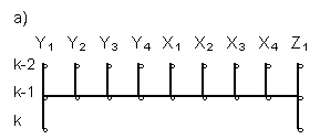
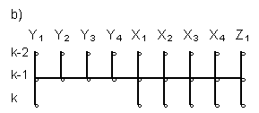
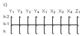
Fig. 1. Patterns:
- explicit, for variable Y1 step-wise forecasting;
- explicit, for normative Y1(k) forecasting;
- implicit for normative of Y1(k) Y2(k)
Y3(k) and Y4(k) forecasting;
Full equations of analogical form were completed for output
variables Y2(k), Y3(k) and Y4(k)
too. Then, using Combinatorial GMDH algorithm, coefficients
for these equations were found. Forecastings were calculated
and their accuracy was evaluated.
An example of normative forecasting
For example, let us consider normative forecasting of Ukraina
macroeconomy on second quarter of 1995 using data presented
in table. Variables having k index will be related to this quarter.
Following values of coefficients were received for the model
forecasting Y1(k) :
a00=-0.823; a11= 0; a122=
0; a20= 0; a21=-1.527; a22=-1.539;
a30= 0; a31= 0.549; a32=
0; a40= 0 a41=-0.120 a42=
0.798
a50= 0 a51= 0 a52= 0.295;
a60= 1.226; a61=-0.800; a62=
0;
a70= 1.311; a71= 0; a72=-0.581;
a80= 0.860; a81= 0; a82=
2.121;
a90= 0.734; a91=-0.467; a92=
2.364
Models accuracy can be characterised by minimal value of RR
criterion. For optimal non-physical forecasting model of Y1(k)
was RRmin=1.59e-14 (MSE=0.0). For forecast
of variable Y2(k) RRmin=7.55e-14
(MSE=3.92e-15); for forecast of Y3(k)
RRmin = 3.63e-5 (MSE=6.77e-6);
and for forecast of Y4(k) RRmin=0.0026
(MSE=1.05e-4). Small minimal value of criterion shows
high accuracy of variable Y1(k) forecasting.
Arguments which have zero coefficient are excluded from model.
This means only that these arguments should be not used for
accurate forecasting. Conclusions about reasonable use of them
for control purposes are not true. For solution of questions
about control the analysis of other, physical model (which us
not considered here) is necessary.
Values of all variables for delayed moments k-1 and k-2 are
known. Substituting them into equations for variables Y1(k),
Y2(k), Y3(k) and Y4(k) for
explicit patterns we receive four separated calculating equations:
Y1(k) = a0 + a1 X1(K)
+ a2 X2(k) + a3 X3(k)
+ a4 X4(k) + a5 Z1(k)
(1)
Y2(k) = b0 + b1 X1(k)
+ b2 X2(k) + b3 X3(k)
+ b4 X4(k) + b5 Z1(k)
(2)
Y3(k) = c0 + c1 X1(k)
+ c2 X2(k) + c3 X3(k)
+ c4 X4(k) + c5 Z1(k)
(3)
Y4(k) = d0 + d1 X1(k)
+ d2 X2(k) + d3 X3(k)
+ d4 X4(k) + d5 Z1(k)
(4)
For equation (1) we receive:
a0=-2.213; a1=0; a2=1.226;
a3=1.311; a4=0.860; a5=0.734
computer algorithm teaches us that to receive accurate normative
forecast of Y1(k) variable is necessary to point
out the values of factors X2(k) X3(k)
and X4(k). For equation (2) we receive:
b0=0.337; b1=0.564; b2=0;
b3=0; b4=1.542; b5=0
For normative forecasting of Y2(k) variable is necessary
to point out factors X1(k) and X4(k).
For equation (3) we receive:
c0=-0.639; c1=0.088; c2=1.477;
c3=0; c4=0; c5=0
For normative forecasting of Y3(k) variable, factors
X1(k) and X2(k) should be pointed out.
At last, for equation (4) we find:
do=0.003; d1=0; d2=0; d3=0.756;
d4=0; d5=0
For the most accurate normative forecasting of Y4(k)
variable should be pointed out only one factor X3(k).
Graphical visualisation of variable Y1(k) normative forecasting
Let us show an example of output variable Y1(k)
normative forecasting visualisation using example considered
above. Let give to variable X4(k) two values:
X4(k) = 0.25 and X4(k) =0.75
The variable Y1(k) change is shown by isolines on
the plane of two input factors X2(k) and X3(k)
(Fig.2a and Fig.2b).
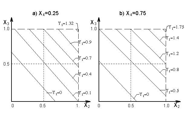
Fig.2. Graphical presentation of variable Y1(k)
forecast.
By comparison of Figures 2a and 2b is possible, particularly,
to conclude that increase of monetary circulation rate leads to
increase of Y1(k); Most important is that using Figures
2a and 2b is possible to establish quantitative connection between
output variable and their input factors. Similar figures can be
completed for each output variable.